what happens if nonlinear features are added to a logistic regression model

Characteristic Scaling — Effectively Choose Input Variables Based on Distributions

Demonstrating how to wisely cull the numerical variables for scaling which results in boosting the accuracy of the model

Photo by Siora Photography on Unsplash

We often run across a state of affairs dealing with a diverseness of numerical variables consisting of different ranges, units, and magnitudes while building an ML model. Equally a common practice, we will apply Standardization or Normalization techniques for all the features earlier building a model. Still, it is crucial to study the distributions of the data before making a decision on which technique to apply for feature scaling.

In this article, we volition get through the departure between Standardization and Normalization along with understanding the distributions of the data. In the end, we will run into how to select the strategies based on Gaussian and Non-Gaussian distribution of the features to improve the performance of the Logistic Regression model.

Standardization Vs Normalization

Both these techniques are sometimes used interchangeably simply they refer to different approaches.

Standardization : This technique transforms the information to have a mean of cypher and a standard difference to 1.

Normalization : This technique transforms the values in variables between 0 and 1.

We are using the Pima Indian Diabetes dataset and you can find the same [here]

            import pandas every bit pd
import numpy as np
data = pd.read_csv("Pima Indian Diabetes.csv")
data.head()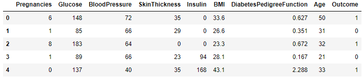          

Beginning few records of the dataset

From the higher up, we tin encounter that the numerical variables are varying in dissimilar ranges and the Outcome is the target variable. We will perform both the scaling techniques and utilise Logistic Regression.

👉 Applying Standardization to all features and modeling.

From the sklearn library, we need to use StandardScaler to implement Standardization.

            from sklearn.preprocessing import StandardScaler
Y = information.Outcome
X = information.drop("Outcome", axis = 1)
columns = X.columns
scaler = StandardScaler()
X_std = scaler.fit_transform(X)
X_std = pd.DataFrame(X_std, columns = columns)
X_std.head()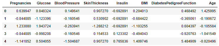          

Transformation of Input features afterwards applying Standardization

Allow us practice the train and examination the split for the standardized features.

            from sklearn.model_selection import train_test_split
x_train, x_test, y_train, y_test = train_test_split(X_std, Y, test_size = 0.15, random_state = 45)          

Now nosotros are going to use Logistic Regression on the standardized dataset.

            #Building Logistic Regression model on the Standardized variables
from sklearn.linear_model import LogisticRegression
lr_std = LogisticRegression()
lr_std.fit(x_train, y_train)
y_pred = lr_std.predict(x_test)
impress('Accuracy of logistic regression on test set with standardized features: {:.2f}'.format(lr_std.score(x_test, y_test)))          

Accurateness of the model with standardized features

From the higher up, nosotros tin come across that the accuracy of the model with all the features applying Standardization technique is 72 pct.

👉 Applying Normalization to all features and modeling.

From the sklearn library, we need to use MinMaxScaler to implement Normalization.

            from sklearn.preprocessing import MinMaxScaler
norm = MinMaxScaler()
X_norm = norm.fit_transform(X)
X_norm = pd.DataFrame(X_norm, columns = columns)
X_norm.head()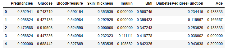          

Transformation of Input features afterwards applying Normalization

Let us do the railroad train and examination the carve up for the normalized features.

            # Train and Test dissever of Normalized features
from sklearn.model_selection import train_test_split
x1_train, x1_test, y1_train, y1_test = train_test_split(X_norm, Y, test_size = 0.15, random_state = 45)          

Applying Logistic Regression on the normalized dataset.

            #Edifice Logistic Regression model on the Normalized variables
from sklearn.linear_model import LogisticRegression
lr_norm = LogisticRegression()
lr_norm.fit(x1_train, y1_train)
y_pred = lr_norm.predict(x1_test)
print('Accuracy of logistic regression on test set with Normalized features: {:.2f}'.format(lr_norm.score(x1_test, y1_test)))          

Accurateness of the model with normalized features

The accuracy of the model when all the features are normalized is 74 pct.

👉 Understanding the distribution of features

Allow u.s. plot the histograms of the variables to report the distribution.

            # Plotting the histograms of each variable
from matplotlib import pyplot
data.hist(blastoff=0.5, figsize=(20, 10))
pyplot.show()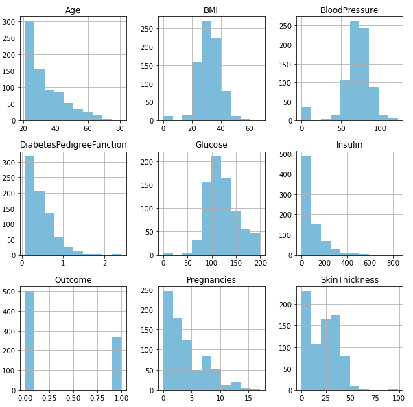          

Histogram for each feature to understand the distribution

Gaussian Distribution — BMI, BloodPressure, Glucose.

Not-Gaussian Distribution — Historic period, DiabetesPedigreeFunction, Insulin, Pregnancies, SkinThickness

👉Normalize Not-Gaussian features and Standardize Gaussian-similar features

Finally, nosotros came to an experiment waiting to select the variables and apply both the strategies based on the distributions on the same dataset.

To apply this strategy, we are going to use Column Transformer and Pipeline concepts from sklearn as we need to practise the mixed blazon of techniques by subsetting the columns.

As mentioned above, we are initiating different pipelines for Gaussian and Non-Gaussian features

            from sklearn.compose import ColumnTransformer
from sklearn.pipeline import Pipeline
              Standardize_Var = ['BMI','BloodPressure', 'Glucose']              
Standardize_transformer = Pipeline(steps=[('standard', StandardScaler())])
              Normalize_Var = ['Age','DiabetesPedigreeFunction','Insulin','Pregnancies','SkinThickness']              
Normalize_transformer = Pipeline(steps=[('norm', MinMaxScaler())])          

At present, let u.s. build the Logistic Regression model on the information with selective features for Standardization and Normalization.

            x2_train, x2_test, y2_train, y2_test = train_test_split(X, Y, test_size=0.2)
              preprocessor = ColumnTransformer(transformers=
                [('standard', Standardize_transformer, Standardize_Var),
                ('norm', Normalize_transformer, Normalize_Var)])                        clf = Pipeline(steps=[('preprocessor', preprocessor),
              ('classifier', LogisticRegression(solver='lbfgs'))])
clf.fit(x2_train, y2_train)
print('Accuracy after standardizing Gaussian distributed features and normalizing Not-Gaussian features: {:.2f}'.format(clf.score(x2_test, y2_test)))          

👉 Concluding key details

Below is the accuracy details for the different models we have congenital so far.

Accurateness after standardizing all the features: 0.72

Accuracy after normalizing all the features: 0.74

Accuracy after applying Standardization to Gaussian distribution features and Normalization to Non- Gaussian distribution features: 0.79

Summary

We need to perform Characteristic Scaling when we are dealing with Slope Descent Based algorithms (Linear and Logistic Regression, Neural Network) and Distance-based algorithms (KNN, K-means, SVM) equally these are very sensitive to the range of the data points. This stride is not mandatory when dealing with Tree-based algorithms.

The main focus of this commodity is to explain how the distribution of the data plays an important part in feature scaling and how to select the strategies based on Gaussian and Non-Gaussian distribution to improve the overall accuracy of the model.

You lot tin can get the complete lawmaking from my GitHub [profile]

Thank y'all for reading and Happy Learning! 🙂

mathewswils1952.blogspot.com

Source: https://towardsdatascience.com/feature-scaling-effectively-choose-input-variables-based-on-distributions-3032207c921f

Share this post